Smart microscopy / translocation assay

Measure EGFP inside nuclei and surrounding rings

DAPI defines the nuclei; the EGFP nucleus-to-ring ratio measures relative nuclear enrichment.

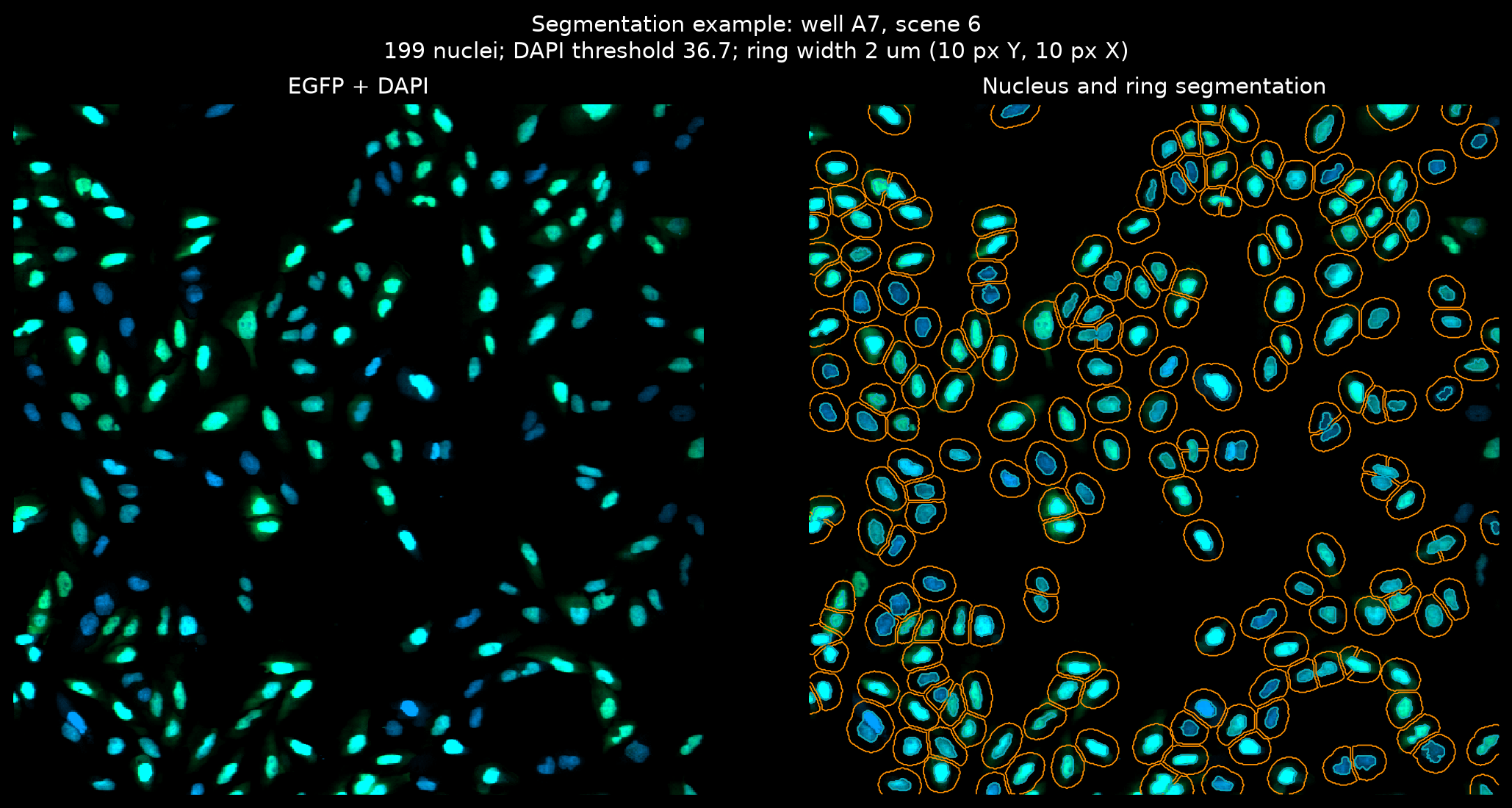
Saved assay plot showing EGFP and DAPI beside detected nucleus and ring boundaries in well A7, scene 6 — Fig. 1The saved field preview pairs the measured fluorescence with nucleus and outer-ring boundaries.

Existing result snapshot, not a new analysis. These Seaborn plots come from results/translocation/notebook_unified_run/transloc_gfp_dapi_0_2micron.czi/. The notebook and CLI share the analysis helpers. Click any plot for full resolution.

Every input uses the same measurement pipeline

Validate and readDetect CZI, OME-Zarr HCS, or OZX. Check plate metadata, channels, scaling, and optional Excel assignments.
Segment nucleiThreshold each DAPI field. Remove small objects, fill holes, and split touching nuclei with watershed.
Measure EGFPBuild outer rings, measure nucleus and ring means, and calculate per-object ratios.
Summarize and fitAggregate wells and doses. Fit increasing Hill curves, export tables, and draw quality-control plots.

CZI supports lazy scene arrays or eager field reads; NGFF reads full-resolution fields without extracting OZX.
The saved run uses Otsu thresholding; other supported global thresholds can be selected.
The ring samples the area around a nucleus; it is not a whole-cell cytoplasm segmentation.
The saved workbook assigns wells to treatments, doses, units, and controls before aggregation.

Fig. 2Input adapters change how fields are read, not how their nuclei and EGFP measurements are analyzed.

The ratio compares a nucleus with its own local ring

Per-object measurement

Mean nuclear EGFPMean ring EGFP

Measure raw intensities, not display-scaled fluorescence.

A non-finite or non-positive ring mean makes the ratio invalid.

Dose response

Cells at or above the ratio cutoffCells with finite ratios

Pool valid cells from replicate treatment wells at each dose.

This is not the same as the median ratio heatmap or an unweighted average of well fractions.

Fig. 3The response counts cells above a ratio cutoff, rather than fitting the plate's median ratios.

The saved preview labels the physical ring width and its pixel equivalent. Rings exclude nuclear pixels and can be truncated by nearby objects or the image boundary.

Read the well assignments before interpreting the heatmaps

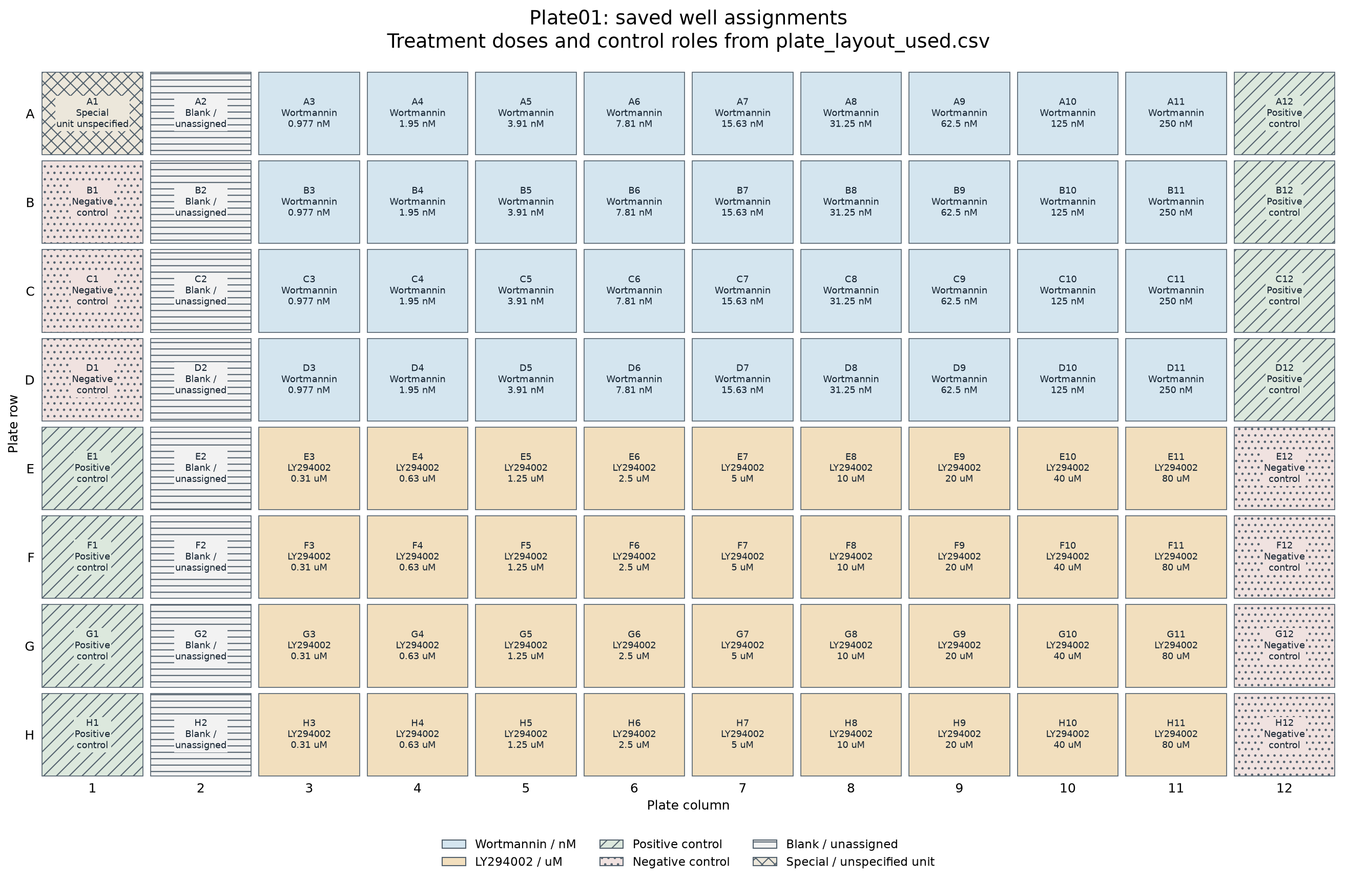
Plate01 well assignments showing treatment names and doses, positive and negative controls, blanks, and the special condition with unspecified unit — Fig. 4The saved plate layout supplies treatment identity, dose, unit, and control roles for each well.

Download the saved well assignments. This layout image is generated from that CSV, not inferred from fluorescence. Special and blank wells remain explicitly labeled; their unspecified doses are not invented.

Controls appear in the well summaries, but only treatment wells with finite doses enter the dose-response table. The normalized fit panels use fitted bottom and top values, not positive-control normalization.

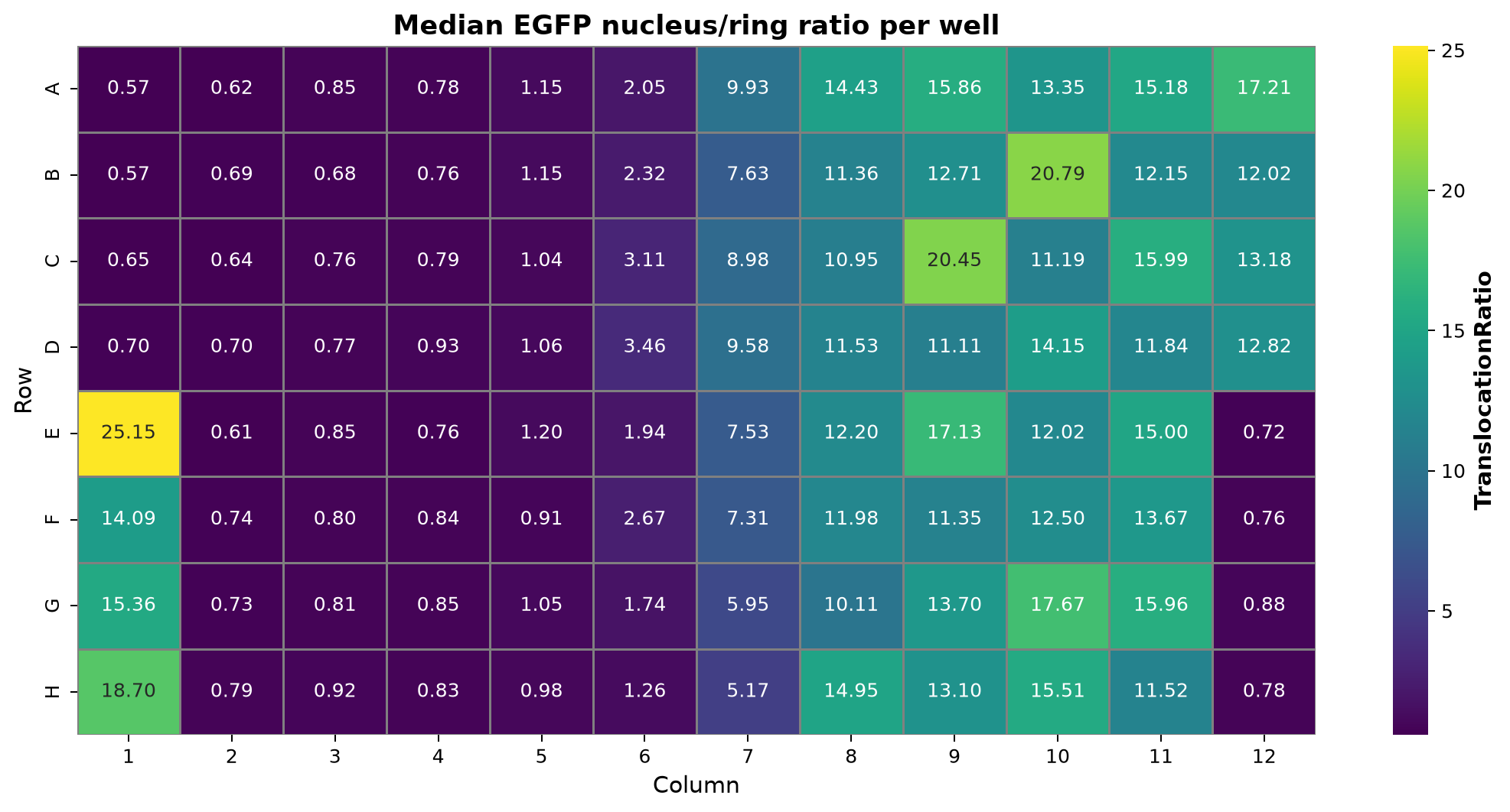
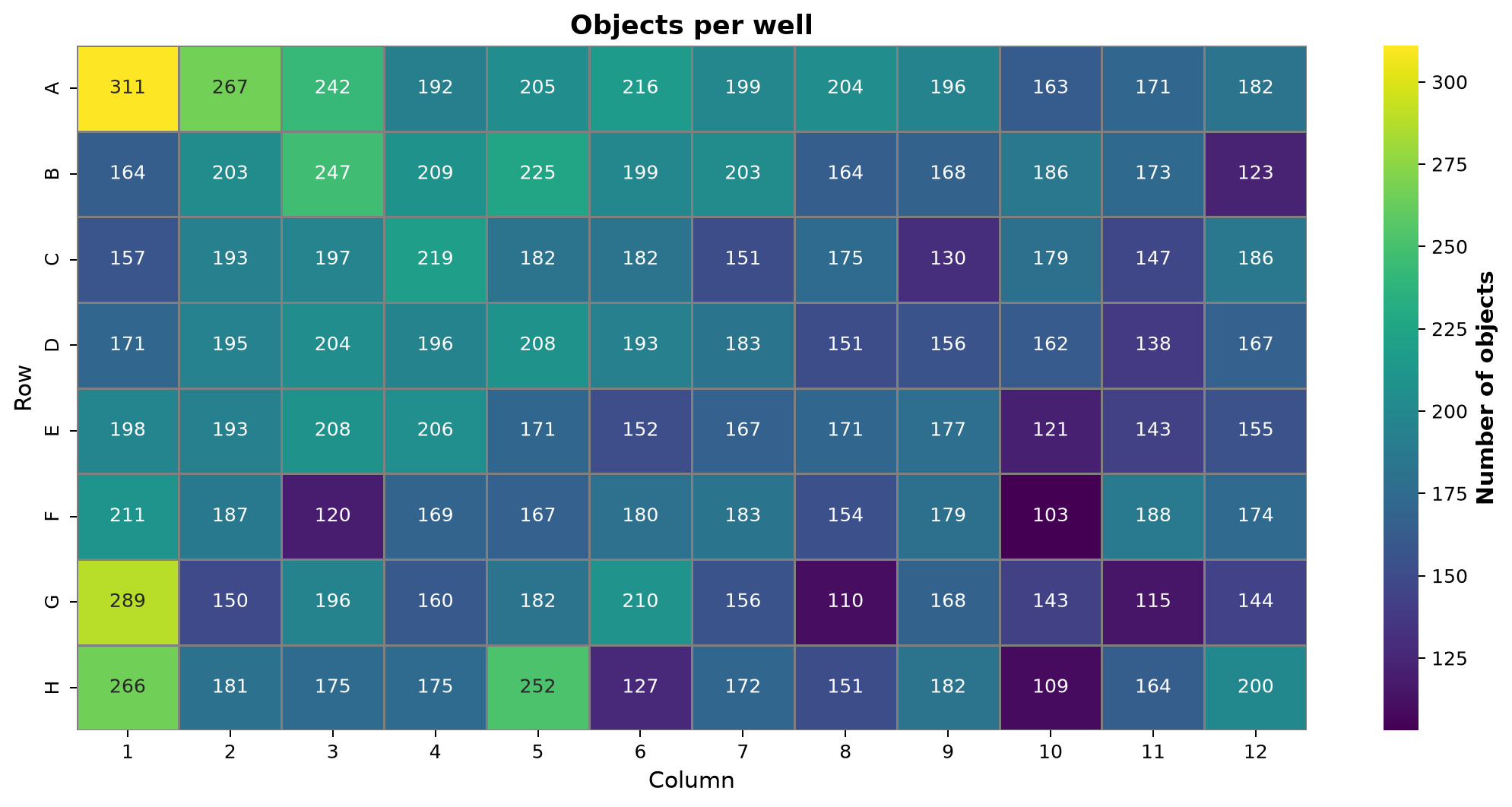
Saved plate heatmap with the median EGFP nucleus-to-ring ratio printed in each well — Fig. 5The median-ratio map shows well-level nuclear enrichment, not the fraction of responding cells.

Saved plate heatmap with the detected object count printed in each well — Fig. 6Object counts expose differences in sampling that a ratio map alone cannot show.

Interpret both maps with the plate assignments and saved well summary; color alone does not establish a treatment effect.

Fit the responding fraction, then inspect the normalized curve

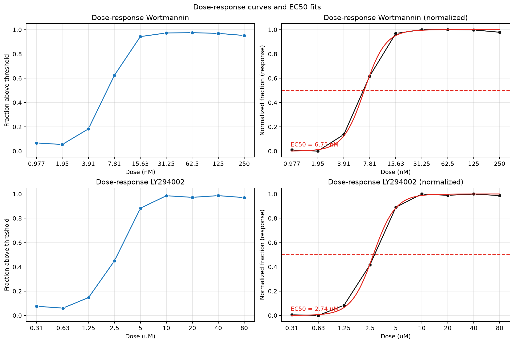
Saved dose-response plots for Wortmannin in nM and LY294002 in micromolar, with raw responding fractions and normalized Hill fits — Fig. 7The saved curves report half-maximal effective concentration estimates for distinct compounds with distinct dose units.

The fit uses a bounded NumPy grid search for an increasing four-parameter Hill curve. The normalized panel subtracts the fitted bottom and divides by the fitted response range.

The estimates are specific to this dataset and segmentation settings, not general compound reference values. Too few finite positive-dose responses or constant responses leave the fit unavailable.

Inspect dose-response values · Inspect fit parameters and status

Keep analysis outputs separate from the published snapshot

New assay run

results/translocation/<run-name>/

Cell measurements, well summaries, dose responses, fit results, field mapping, and analysis parameters.

When using an Excel layout, also save the assignments used for the run.

This documentation snapshot

examples/translocation/translocation_docs/

The editable source, rendered walkthrough, copied plots, and compact supporting CSVs live together.

No links depend on ignored result folders. Rerunning the assay does not refresh these copied plots.

Fig. 8The documentation includes its own plot assets so GitHub Pages does not need the local results directory.

cd /d "F:\Pixi_Projects\zen_czi\smartmicroscopy"
pixi run --locked -e default python "examples\translocation\translocation_assay.py" ^
  --input "data\transloc_gfp_dapi_0_2micron.czi" ^
  --plate-layout "data\plate_layout_example.xlsx" ^
  --output-dir "results\translocation\visual-example" ^
  --plot-backend seaborn

CMD uses ^ for continuation, with no trailing spaces. Select an unused output folder to retain earlier results. The command illustrates the CLI; it did not create the snapshot shown above.

Seaborn writes static PNGs. The CLI defaults to Plotly for interactive HTML. Omit --plate-layout only when the built-in assignments match the sample.

The field loop feeds well summaries and dose fits

Fig. 9The code aggregates object measurements only after processing all mapped fields, and records unavailable fits instead of inventing EC50 values.

Editable Mermaid flowchart. Validation and read errors stop the analysis; they are not successful empty results.

Follow the functions and edge cases

main() and run_analysis() parse options, reject incompatible ring-width settings, load input metadata, and enforce channel order EGFP then DAPI. prepare_scene_inputs() supplies either lazy scenes or a field-reader callback.

analyze_scenes() loads each mapped field, checks matching channel planes, and calls the segmentation and measurement helpers. Fields without nuclei produce no cell rows; they still contribute field and threshold bookkeeping.

make_ring_labels() uses nearest-nucleus distance to assign background pixels, then removes pixels touching a different nucleus or ring label. measure_scene_objects() uses label-wise pixel sums and areas; an empty ring or invalid ring mean yields a non-finite ratio.

summarize_wells() combines fields by well. dose_response_table() pools finite cell ratios from matching treatment wells rather than averaging their medians. fit_hill() rejects too few usable dose responses or a constant response and records the reason.

write_analysis_outputs() writes cell, well, dose, and fit tables plus plots and parameters. run_analysis() separately writes field_mapping.csv and, when an Excel layout is supplied, plate_layout_used.csv.

Sources and provenance

Assay README · CLI and orchestration · Segmentation, measurements, fitting, and plotting · Input adapters · Plate assignments

Plot snapshot: transloc_gfp_dapi_0_2micron.czi, from the existing unified notebook run. Saved parameters select Otsu, the Excel plate layout, channel order EGFP then DAPI, and Seaborn output. The segmentation image itself labels its field, threshold, ring width, and object count.

Editable visual source. Source review and existing result inspection only; no new assay was run for this page.